Backpropagation (My fav)
November 12, 2025
Welcome, this is part of my series posts where I explain ML concepts. I assume that you have already taken calculus 1, if you understand the chain rule, good! One thing to note, I won’t be going over gradient descent itself much here, I have another post outlining the theory behind gradient descent in the context of a simpler model.
Here, I’ll be going over the math of backpropagation, only briefly touching on the high level intuition since there are better sources for that.
As always, I give my thanks to 3Blue1Brown (Grant) for the amazing videos.
Notation
A quick note on notation before we dive in:
- I use both subscripts and superscripts to signify layer, but it should be clear from context
- \(J()\) signifies the cost function, and \(C\) represents the output of the cost function (the cost itself)
- \(\hat{y}\) is our prediction — it’s also equal to the last activation value \(a^L\) in the neural network
- \(g\) = ReLU (activation function for hidden layers)
- \(\sigma\) = sigmoid (activation function for output layer, or softmax if multiclass)
Intuitive Motivation for Backpropagation
So, Backpropagation is the backwards movement through a neural network’s nodes to gauge how much each weight contributes to the overall cost.
By finding out how each weight contributes to the cost, we can adjust the weights accordingly to most efficiently lower cost.
The best way to see how much a weight’s value changes the overall cost would be to change the value of a particular weight (say, \(\theta_1\)) and observe the resulting change in cost.
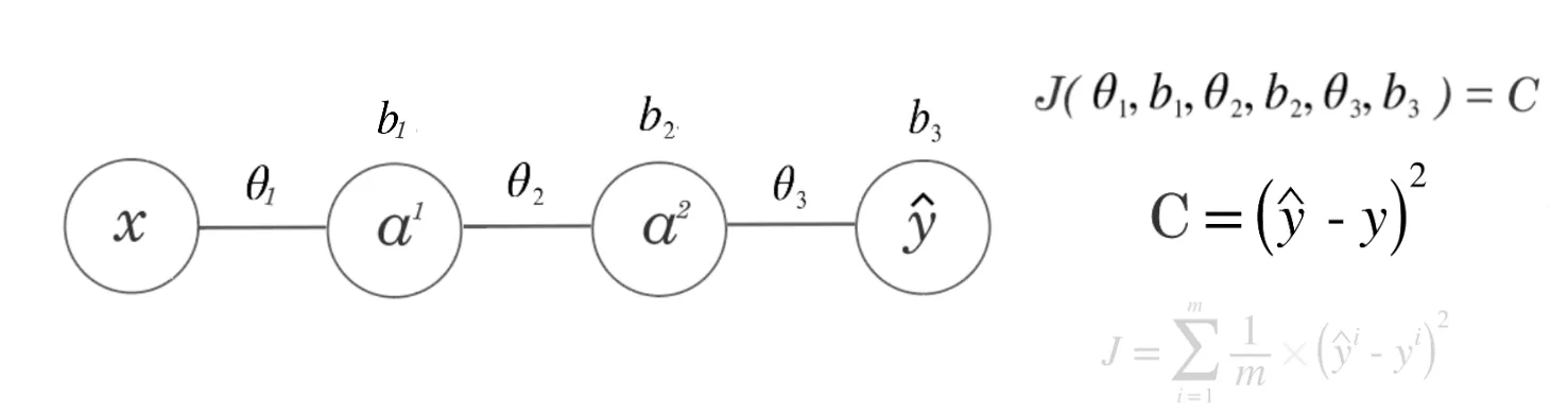
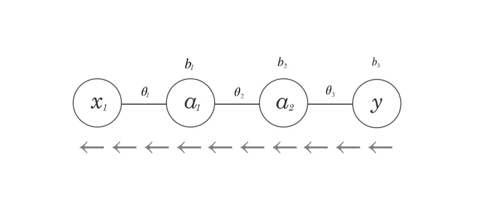 This NN has two hidden layers, three weights, and three biases.
The cost function takes in all these parameters:
\[ J(\theta_1, b_1, \theta_2, b_2, \theta_3, b_3) = C \]
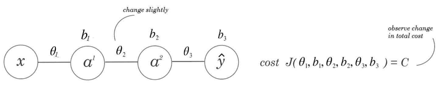
The ratio of the change in \(\theta_2\) and the resulting change in \(C\) would be the perfect indicator of each weight’s impact on the cost:
- Weights with higher ratios (where the change in \(C\) is much larger than the change in \(\theta\)) have large sway on the cost
- Weights with lower ratios have less importance in deciding cost
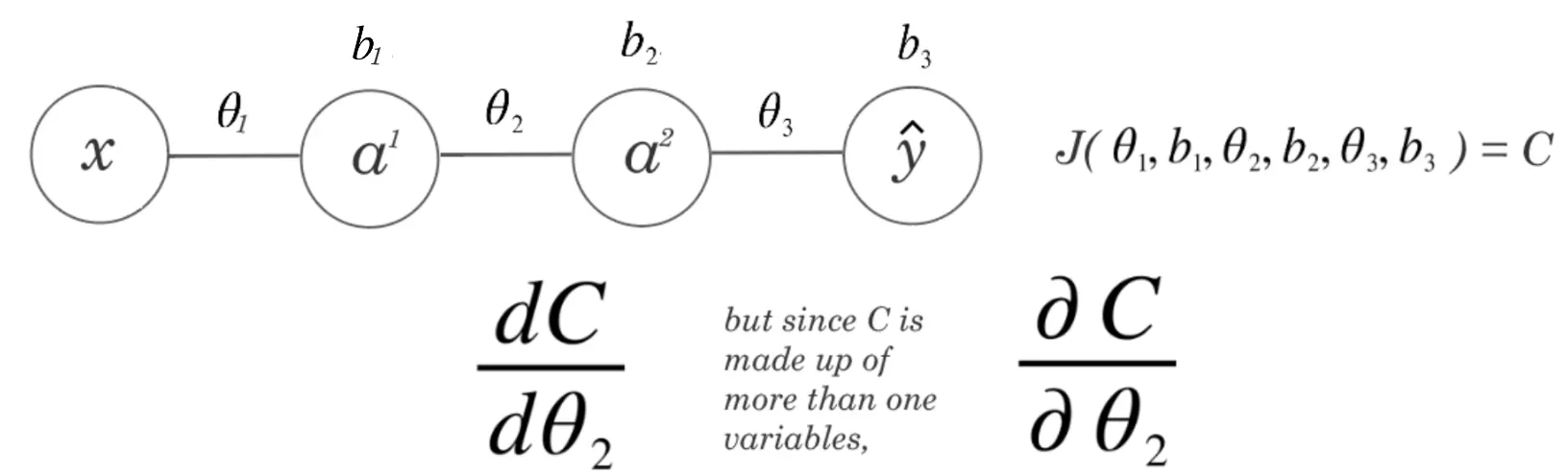
There’s a reason why calc knowledge is important, This sounds like a derivative.
\[ \frac{dC}{d\theta_2} \quad \text{but since } C \text{ is made up of more than one variable,} \quad \frac{\partial C}{\partial \theta_2} \]
We need to find a way to cycle through every weight and bias in our network and calculate the partial derivative with the cost function:
\[ \frac{\partial C}{\partial \theta_1}, \quad \frac{\partial C}{\partial b_1}, \quad \frac{\partial C}{\partial \theta_2}, \quad \frac{\partial C}{\partial b_2}, \quad \frac{\partial C}{\partial \theta_3}, \quad \frac{\partial C}{\partial b_3} \]
Then, as I explain in my gradient descent article, we can update every weight and bias by its corresponding partial derivative, which will shift the entire network to something with slightly lower cost.
The Chain Rule in Backpropagation
It’s hard to overstate the importance of the chain rule in backpropagation. In fact, backpropagation is just the chain rule executed in sequence.
\[ \frac{dy}{dx} = \frac{dy}{du} \cdot \frac{du}{dx} \]
The chain rule finds the derivative of composite functions, which is a function inside another function, like \(f(g(x))\). Even though it’s most commonly seen with a pair of functions, the chain rule extends to functions with many compositions, like \(a(b(c(d(e(f(g(x)))))))\). We just have to multiply more derivatives:
\[ \frac{da}{dx} a(b(c(d(e(f(g(x))))))) \]
\[ \frac{da}{\partial x} = \frac{da}{db} \times \frac{db}{dc} \times \frac{dc}{dd} \times \frac{dd}{de} \times \frac{de}{df} \times \frac{df}{dg} \times \frac{dg}{dx} \]
We can think of our neural network as one big composite function. The cost \(C\) is the final output. In between, we have many smaller functions.
Forward Propagation as Composition
If we think back to forward propagation, we’re essentially calculating a string of composite functions, composing \(z\)’s and \(g\)’s inside each other. Each layer depends on the outputs of the last.
\[ z^1 = \theta^T x + b^1 \] \[ a^1 = g(z^1) \] \[ z^2 = \theta^T a^1 + b^2 \] \[ \vdots \] \[ a^L = \sigma(z^L) \] \[ \hat{y} = a^L \] \[ C = J(\hat{y}, y) \]
So finding the derivatives of the cost function is like finding the derivatives of a big composite function. And this is where backpropagation comes from.
- The NN is a series of composed functions.*
Just like how we start from the outside when differentiating composite functions (closest to the output), we start from the “outside” of our neural network, where we have \(J()\), which encompasses all the little functions inside.
\[ \frac{\partial}{\partial x} C\left(\hat{y}\left(z^3\left(a^2\left(z^2\left(a^1\left(z^1(x)\right)\right)\right)\right)\right)\right) \]
The Backpropagation Paths
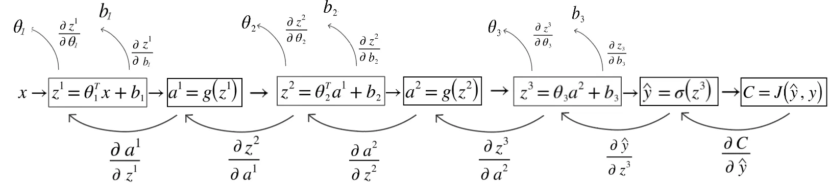 All the partial derivatives we need to compute, shown as arrows going backwards.
We can identify the specific derivative “paths” we have to take to get to each of our weights and biases, starting at the cost. We traverse these paths backwards while keeping chain rule intact.
For a network with three layers, here are all six partial derivatives we need:
\[ \frac{\partial C}{\partial \theta_1} = \frac{\partial z^1}{\partial \theta_1} \cdot \frac{\partial a^1}{\partial z^1} \cdot \frac{\partial z^2}{\partial a^1} \cdot \frac{\partial a^2}{\partial z^2} \cdot \frac{\partial z^3}{\partial a^2} \cdot \frac{\partial \hat{y}}{\partial z^3} \cdot \frac{\partial C}{\partial \hat{y}} \]
\[ \frac{\partial C}{\partial b_1} = \frac{\partial z^1}{\partial b_1} \cdot \frac{\partial a^1}{\partial z^1} \cdot \frac{\partial z^2}{\partial a^1} \cdot \frac{\partial a^2}{\partial z^2} \cdot \frac{\partial z^3}{\partial a^2} \cdot \frac{\partial \hat{y}}{\partial z^3} \cdot \frac{\partial C}{\partial \hat{y}} \]
\[ \frac{\partial C}{\partial \theta_2} = \frac{\partial z^2}{\partial \theta_2} \cdot \frac{\partial a^2}{\partial z^2} \cdot \frac{\partial z^3}{\partial a^2} \cdot \frac{\partial \hat{y}}{\partial z^3} \cdot \frac{\partial C}{\partial \hat{y}} \]
\[ \frac{\partial C}{\partial b_2} = \frac{\partial z^2}{\partial b_2} \cdot \frac{\partial a^2}{\partial z^2} \cdot \frac{\partial z^3}{\partial a^2} \cdot \frac{\partial \hat{y}}{\partial z^3} \cdot \frac{\partial C}{\partial \hat{y}} \]
\[ \frac{\partial C}{\partial \theta_3} = \frac{\partial z^3}{\partial \theta_3} \cdot \frac{\partial \hat{y}}{\partial z^3} \cdot \frac{\partial C}{\partial \hat{y}} \]
\[ \frac{\partial C}{\partial b_3} = \frac{\partial z^3}{\partial b_3} \cdot \frac{\partial \hat{y}}{\partial z^3} \cdot \frac{\partial C}{\partial \hat{y}} \]
Notice the pattern here: weights closer to the output have shorter chains, while weights closer to the input require multiplying through more derivatives.
Computing Backprop with Squared Error Cost
Let’s work through an example. Our cost function is squared error:
\[ C = (\hat{y} - y)^2 \]
For multiple training examples, this becomes:
\[ J = \sum_{i=1}^{m} \frac{1}{m} \times (\hat{y}^i - y^i)^2 \]
Since we’re dealing with a single training example for clarity, we only need to think about the loss of a single point.
Let’s compute \(\frac{\partial C}{\partial \theta_2}\). The path we need to follow is:
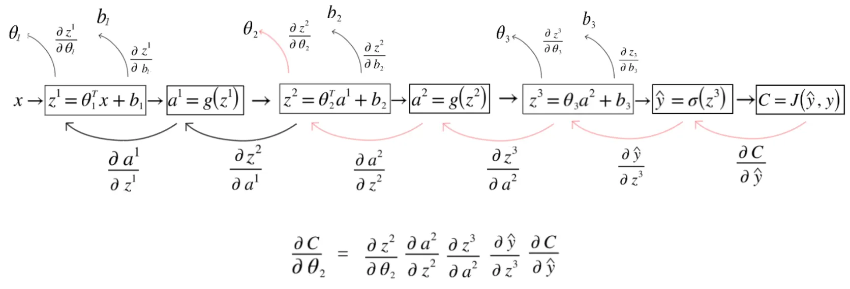
\[ \frac{\partial C}{\partial \theta_2} = \frac{\partial z^2}{\partial \theta_2} \cdot \frac{\partial a^2}{\partial z^2} \cdot \frac{\partial z^3}{\partial a^2} \cdot \frac{\partial \hat{y}}{\partial z^3} \cdot \frac{\partial C}{\partial \hat{y}} \]
Let’s go backwards from \(C\).
Step 1: Derivative of Cost w.r.t \(\hat{y}\)
First, we need the derivative of our cost w.r.t our prediction \(\hat{y}\):
\[ C = (\hat{y} - y)^2 \]
\[ \frac{\partial C}{\partial \hat{y}} = \frac{\partial}{\partial \hat{y}} (\hat{y} - y)^2 = 2(\hat{y} - y) \times \frac{\partial \hat{y}}{?} \]
The question mark represents: what is the input into \(\hat{y}\) that helps us travel further back into the network?
Note: \(\hat{y}\) is a function made up of more “parts” where the weights and activations of previous layers. This means we must use the chain rule.
Step 2: Derivative w.r.t \(z^3\) (The Sigmoid Derivative)
\(\hat{y}\) has just one input: \(z^3\). Since \(\hat{y} = \sigma(z^3)\), we must find the derivative of sigmoid.

\[ \frac{\partial C}{\partial z^3} = 2(\hat{y} - y) \times \frac{\partial \hat{y}}{\partial z^3} \]
\[ = 2(\hat{y} - y) \times \frac{\partial}{\partial z^3} \sigma(z^3) \]
\[ = 2(\hat{y} - y) \times \frac{\partial}{\partial z^3} \frac{1}{1 + e^{-z^3}} \]
Here’s the full derivation of the sigmoid derivative:
\[ = 2(\hat{y} - y) \times \frac{\partial}{\partial z^3} (1 + e^{-z^3})^{-1} \]
\[ = 2(\hat{y} - y) \times -(1 + e^{-z^3})^{-2} \times \frac{\partial}{\partial z^3}(1 + e^{-z^3}) \]
\[ = 2(\hat{y} - y) \times -(1 + e^{-z^3})^{-2} \times (-e^{-z^3}) \]
\[ = 2(\hat{y} - y) \times \frac{e^{-z^3}}{(1 + e^{-z^3})^2} \]
\[ = 2(\hat{y} - y) \times \frac{1}{1 + e^{-z^3}} \times \frac{e^{-z^3}}{1 + e^{-z^3}} \]
\[ = 2(\hat{y} - y) \times \frac{1}{1 + e^{-z^3}} \times \frac{(1 + e^{-z^3}) - 1}{1 + e^{-z^3}} \]
\[ = 2(\hat{y} - y) \times \frac{1}{1 + e^{-z^3}} \times \left(1 - \frac{1}{1 + e^{-z^3}}\right) \]
\[ = 2(\hat{y} - y) \times \sigma(z^3)(1 - \sigma(z^3)) \]
The sigmoid derivative simplifies beautifully to \(\sigma(z)(1-\sigma(z))\)!
Step 3: Derivative w.r.t \(a^2\)
Next, we compute the derivative of \(z^3\) with respect to \(a^2\). Since \(z^3 = \theta_3 a^2 + b_3\):
\[ \frac{\partial z^3}{\partial a^2} = \frac{\partial}{\partial a^2}(\theta_3 a^2 + b_3) = \theta_3 \]
So:
\[ \frac{\partial C}{\partial a^2} = 2(\hat{y} - y) \times \sigma(z^3)(1 - \sigma(z^3)) \times \frac{\partial z^3}{\partial a^2} \]
\[ \frac{\partial C}{\partial a^2} = 2(\hat{y} - y) \times \sigma(z^3)(1 - \sigma(z^3)) \times \theta_3 \]
Each term corresponds to a partial derivative in the chain:
- \(2(\hat{y}-y)\) is \(\frac{\partial C}{\partial \hat{y}}\)
- \(\sigma(z^3)(1-\sigma(z^3))\) is \(\frac{\partial \hat{y}}{\partial z^3}\)
- \(\theta_3\) is \(\frac{\partial z^3}{\partial a^2}\)
Step 4: Derivative w.r.t \(z^2\)
Continuing down the line, we pass through our second activation function:
\[ \frac{\partial C}{\partial z^2} = \frac{\partial C}{\partial \hat{y}} \times \frac{\partial \hat{y}}{\partial z^3} \times \frac{\partial z^3}{\partial a^2} \times \frac{\partial a^2}{\partial z^2} \]
\[ \frac{\partial C}{\partial z^2} = 2(\hat{y} - y) \times \sigma(z^3)(1 - \sigma(z^3)) \times \theta_3 \times g’(z_2) \]
Where \(g’(z_2)\) is the derivative of the ReLU activation function.*
Note: ReLU isn’t technically differentiable at exactly 0, but we can still use it since landing on exactly 0.000… is rare, and implementations just shift it slightly.
Step 5: Finally, \(\theta_2\)!
Now we can “branch off” and calculate our derivative w.r.t \(\theta_2\).
Now that we have \(\frac{\partial C}{\partial z^2}\), we can compute the final piece:
\[ \frac{\partial}{\partial \theta_2} z^2 = \frac{\partial}{\partial \theta_2}(\theta_2^T a^1 + b_2) \]
\[ \frac{\partial z^2}{\partial \theta_2} = a^1 \]
It’s interesting to note that the derivative of the weight is just the activation of the previous layer, showing that weights are only important in proportion to the activations.
The Final Answer
\[ \frac{\partial C}{\partial \theta_2} = 2(\hat{y} - y) \times \sigma(z^3)(1 - \sigma(z^3)) \times \theta_3 \times g’(z_2) \times a^1 \]
Breaking down each term:
- \(\frac{\partial C}{\partial \hat{y}} = 2(\hat{y}-y)\)
- \(\frac{\partial \hat{y}}{\partial z^3} = \sigma(z^3)(1-\sigma(z^3))\)
- \(\frac{\partial z^3}{\partial a^2} = \theta_3\)
- \(\frac{\partial a^2}{\partial z^2} = g’(z_2)\)
- \(\frac{\partial z^2}{\partial \theta_2} = a^1\)
The Bias \(b_2\)
It’s pretty easy to also get the bias:
\[ \frac{\partial}{\partial b_2} z^2 = \frac{\partial}{\partial b_2}(\theta_2^T a^1 + b_2) \]
\[ \frac{\partial z^2}{\partial b_2} = 1 \]
So the derivative w.r.t \(b_2\) is just everything we computed for \(\theta_2\), but with 1 instead of \(a^1\) at the end.
Remember what this is doing. This line of mathematics backpropagates through the neural network, from the cost towards the input. This product is the result of using chain rule to go further through the network by using previously computed numbers.
You can easily follow this same logic to find any weight or bias in the entire system, by calculating the chain rule to access weights that are farther and farther away from the cost.
The key insight is that we reuse computations. Once we’ve computed \(\frac{\partial C}{\partial z^3}\), we don’t need to recompute it when finding \(\frac{\partial C}{\partial \theta_2}\) or \(\frac{\partial C}{\partial b_2}\). This is what makes backpropagation efficient.
We’re done
Backpropagation is really just the chain rule applied systematically through a neural network.
The elegance lies in how we can compute gradients for millions of parameters by simply:
- Going forward to compute all the \(z\)’s and \(a\)’s
- Going backward, multiplying derivatives as we go
- “Branching off” at each layer to grab the weight and bias gradients
This is how neural networks learn. This is how machines learn from data.