Calibrating Volatility Smile Parameters
November 22, 2025
Hello, as exams come close and thanksgiving break is around the corner (Not really a break sadly). I’ve been revisiting a project on trying to figure out how to price options in a way that goes beyond just assuming the midprice is fair value. In illiquid options with wide spreads, the midprice doesn’t really tell you much, it just stems from where the bid and ask happen to be placed.
My goal was to build a lightweight SABR like model to figure out if certain strikes are under or overpriced, or maybe even see if there’s mispricings in the tails. The actual smile just shows the current state but doesn’t provide information on relative over/underpricings.
I came across a paper by Frido Rolloos called “The ATM implied volatility slope, the (dual) volatility swap, and the (dual) zero vanna implied volatility” that connects the ATM implied volatility slope to volatility swap prices.
The Core Equation
The paper gives us a relationship between the implied volatility smile and three parameters: \(\sigma\) (instantaneous volatility), \(\eta\) (vol of vol), and \(\rho\) (correlation between spot and volatility).
Let \(v = \text{vanna}\) and \(w = \text{vomma}\). The key equation is:
\[ \frac{1}{2}\Gamma^{BS}S^2(\sigma^2-\Sigma^2)+\frac{1}{2}w^{BS}\Sigma^2\eta^2+v^{BS}S\Sigma\eta\sigma\rho = 0 \]
Where:
- \(\Gamma^{BS}\) is the Black-Scholes gamma
- \(v^{BS}\) is vanna (sensitivity of delta to volatility)
- \(w^{BS}\) is vomma (sensitivity of vega to volatility)
- \(S\) is the underlying price
- \(\Sigma\) is the implied volatility
The idea is that given market data (gamma, vanna, vomma from the options chain), we can solve for the model parameters that make this equation hold. The formula itself is pretty straightforward.
Solving for the Parameters
Rearranging the equation, we can solve for each parameter:
\[ \sigma = \pm \frac{\left(\sqrt{\Sigma^2 S^2 (\Gamma^2 S^2 + \rho^2 v^2 \eta^2 - \Gamma w\,\eta^2)}-\Sigma \rho\eta S v\right)}{\Gamma S^2}, \quad \Gamma S \neq 0 \]
\[ \eta = \pm \frac{\left(\sqrt{\Sigma^2 S^2 (\rho^2\sigma^2 v^2 + \Gamma w(\Sigma^2 - \sigma^2))}-\Sigma\rho\sigma S v\right)}{\Sigma^2 w}, \quad \Sigma w \neq 0 \]
\[ \rho = \frac{\Gamma S^2(\Sigma^2-\sigma^2)-\Sigma^2\eta^2 w }{2 \Sigma\sigma\eta S v }, \quad \Sigma\sigma\eta S v \neq 0 \]
My Implementation
I pulled SPX options data and computed the greeks.
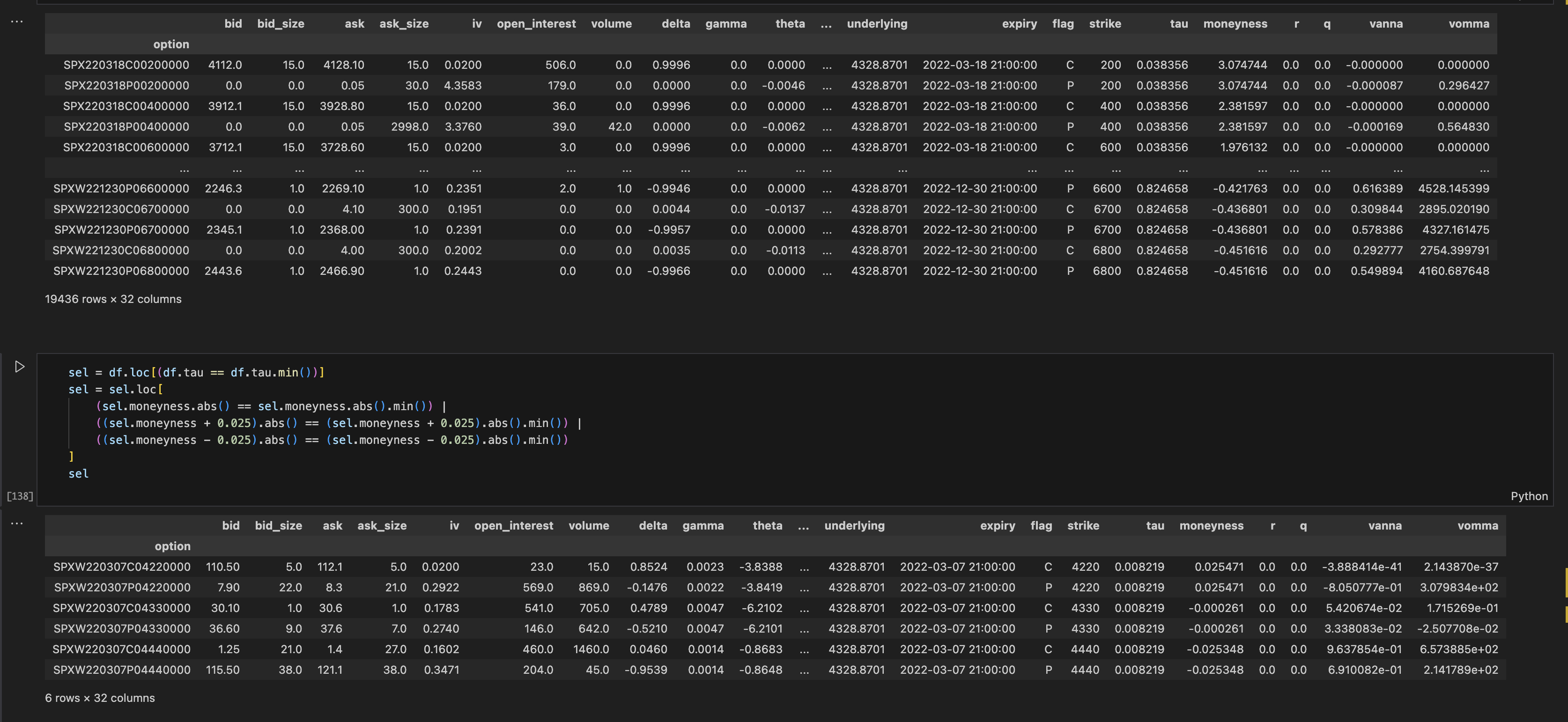 The full SPX options chain with computed greeks including vanna and vomma.
My approach was to select ATM options and nearby strikes (around \(\pm 2.5\%\) moneyness) from the shortest expiry, then try to calibrate \(\sigma\), \(\eta\), and \(\rho\) by minimizing the squared error of the equation above.
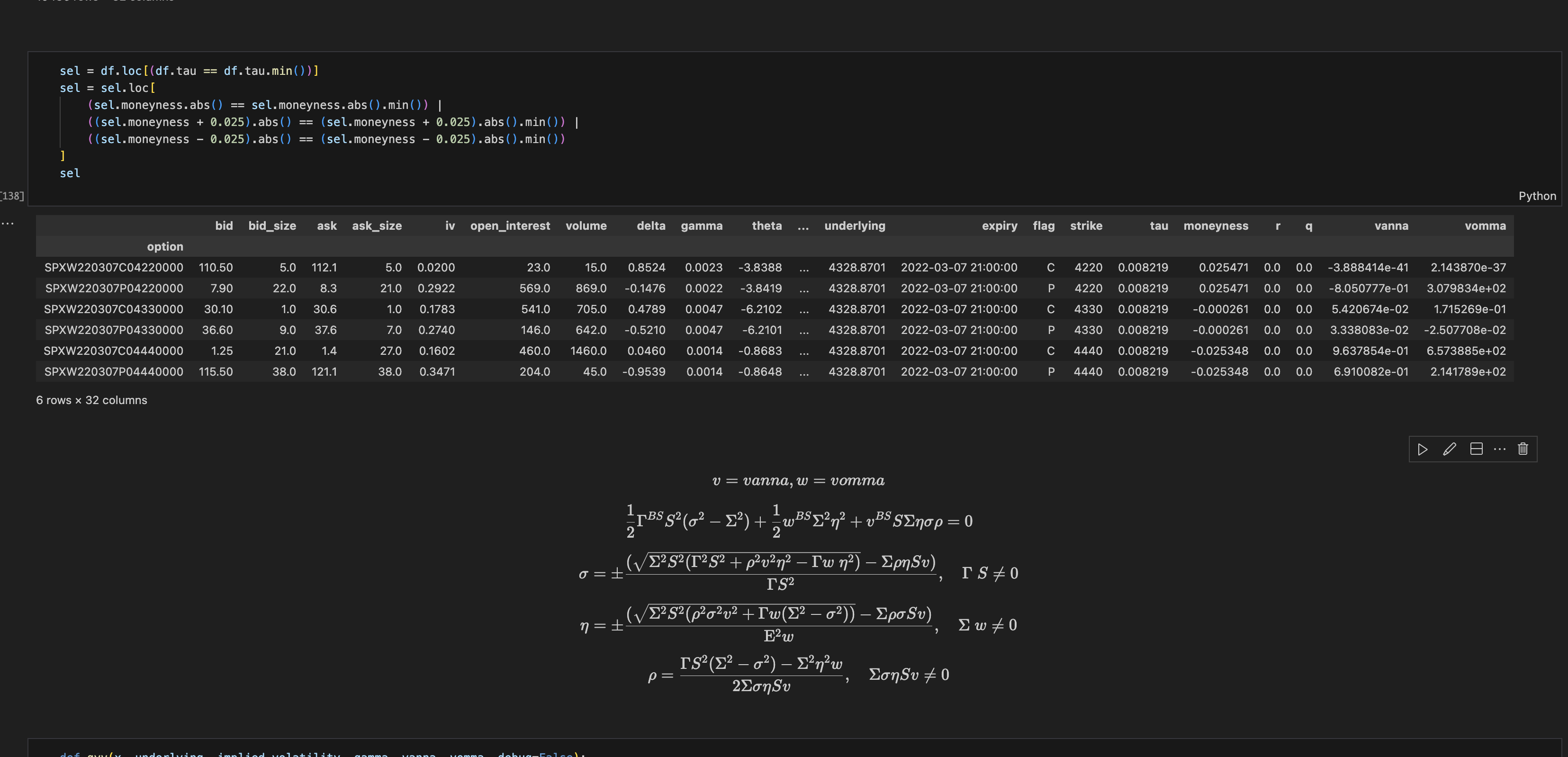 Filtering to ATM and near-ATM options for calibration, with the key equations.
def gvv(x, underlying, implied_volatility, gamma, vanna, vomma):
    sigma, eta, rho = x
    S, epsilon = underlying, implied_volatility

    gamma_part = 0.5 * gamma * S ** 2 * (sigma ** 2 - epsilon ** 2)
    vanna_part = vanna * S * epsilon * eta * sigma * rho
    vomma_part = 0.5 * vomma * epsilon ** 2 * eta ** 2

    return np.mean((gamma_part + vanna_part + vomma_part) ** 2)

bounds = [(0, None), (0, None), (0, None)]
result = minimize(
    gvv,
    [0, 1, 0],
    args=(curr.underlying, curr.iv, curr.gamma, curr.vanna, curr.vomma),
    bounds=bounds,
    options={"maxiter": 1000}
)
The Problems I Ran Into
The equation is supposed to equal zero. But when I plugged in my calibrated parameters and checked each option individually, I got residuals all over the place:
contractSymbol
SPY220307C00432000    26.693284
SPY220307C00441000     0.082834
SPY220307P00432000   -30.577201
SPY220307P00418000    -0.053906
Definitely not zero.
I thought maybe I could go the other way: calibrate sigma, eta, and rho with the wings and back out the prices for ATM. But that didn’t work either.
Issue 1: The model doesn’t see what the market sees
I learned that these stochastic volatility models are usually good for valuing exotics in a way that’s consistent with the vanilla curve. But for actually trading vanillas against other bits of the curve? Probably not good enough. The model doesn’t capture everything the market is pricing in.
Issue 2: Maybe this is only useful for illiquids
I don’t think this approach is very applicable to liquid options. But I see the use case in illiquid options with wide spreads, to at least get an idea of fair price instead of just assuming midprice. I’ve heard from an options market maker on a podcast (Flirting with Models) that they are sometimes themselves not sure about fair price if there is very little traded, and just assume midprice and quote large spreads. So maybe there’s something to be had there. It won’t be a lot, so it’s unlikely to attract larger players, but maybe for retail it’s interesting.
Issue 3: Market makers do NO pricing
I realized that market makers do no pricing. Any real theo price operates at a much longer time scale than the bid ask collection process. They have theo values but these are just midpoints of the bid ask. In illiquid stuff almost any “model” works. In liquid ones hardly no model does, but you have so many strikes it doesn’t matter.
The approach that actually works? Pricing based on historical return distributions, this is why Monte Carlo is popular because it allows atypical return distributions, normal distributions are nice to work with but aren’t rooted in reality.
What Actually Matters
Here’s what I took away from all this:
Getting a good ATM vol estimate is 90% of the work. In the same way that directional trading won’t work if you can’t forecast vol, skew trading won’t work either. And getting a good ATM vol needs more than just history, you need to estimate what it should be relative to future realized vol. That risk premium is time varying and often mispriced.
It’s less about backing out the price of the option and more about estimating RV and IV. You estimate the overall level, then pick the best option out of your set. This is more in the realm of GARCH models, less so BSM.
If you want an actual estimate of fair value of an option, a market maker would be one of the last people to ask. Their job is to manage inventory and capture spread, not to have opinions on fair value.
What I Learned
-
Stochastic vol models like SABR are for pricing exotics consistently with the vanilla curve, not for trading vanillas against each other.
-
Monte Carlo with historical return distributions beats trying to calibrate a parametric model to the current smile. It requires less fussing over parameters.
-
The actual smile just shows the current state — it doesn’t directly tell you about relative over/underpricing. You need a view on future RV to have an opinion.
-
Illiquid options might be where fair value models are useful but even there, the edge is small.
-
90% of the effort should go into estimating ATM vol correctly. Everything else follows from that.
The math is elegant, but the practical application for vanilla options just isn’t there. Maybe I’ll revisit it someday.