Monte Carlo Methods Walkthough
November 25, 2025
Monte Carlo methods are simple but powerful for numerical integration. My post on this would be going over a few variance reduction techniques that can make our estimators less noisy, with antithetic sampling, control variates, and stratified sampling. Before we dive in, let’s talk about why variance matters in a few real world contexts so we can build intuition. It’s always important in my book to build that first for anything.
Quantitative Finance
In finance, we simulate expected returns on our books by sampling over all possible movements in the market. Certain rare events (for example, a terrorist attack) are highly unlikely but have such a big impact on the economy that we want to account for it in our expectation. Modeling these “black swan” events are of considerable interest to financial industries.
Deep Learning
In minibatch stochastic gradient descent, we compute the parameter update using the expected gradient of the total loss across the training dataset. It takes too long to consider every point in the dataset, so we estimate gradients with stochastic minibatch. This is nothing more than a monte carlo estimate.
\[ E_x[\nabla_\theta J(x; \theta)] = \int p(x) \nabla_\theta J(x; \theta) dx \approx \frac{1}{m} \sum_i^m \nabla_\theta J(x_i; \theta) \]
The less variance we have, the sooner our training converges.
Computer Graphics
When it comes to rendering, we are trying to compute the total incoming light arriving at each camera pixel. The vast majority of paths contribute zero radiance, thus making our samples noisy. Decreasing variance allows us to “de-speckle” the pictures.
\[ \mathcal{L}(x, \omega_o) = \mathcal{L}e(x, \omega_o) + \int{\Omega} f_r(x, \omega_i, \omega_o) \mathcal{L}(x’, \omega_i)(\omega_o \cdot n_x) \, d\omega_i \]
\[ \approx \mathcal{L}e(x, \omega_o) + \frac{1}{m} \sum{i}^{m} f_r(x, \omega_i, \omega_o) \mathcal{L}(x’, \omega_i)(\omega_o \cdot n_x) \]
The Problem
Our goal is to find the EV of the random variable \(X\):
\[ X = f(u) = \exp(\sin(8u_1^2 + 3u_1) + \sin(11u_2)) \]
where \(u\) is a 2D point sampled uniformly from the unit square.
f(x,y) = exp(sin(8x.^2+3x)+sin(11y))
plot(linspace(0,1,100),linspace(0,1,100),f,st=:contourf,title="f(X)",size=(400,400))
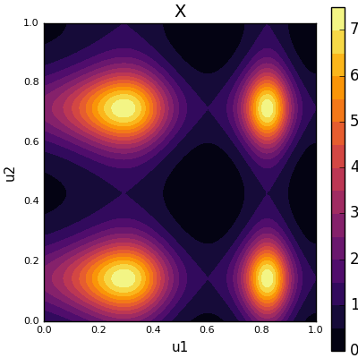 Our function f(X) over the unit square
The expectation can be rewritten as an integral over the unit square like this
\[ \mathbb{E}[X] = \int_0^1 \int_0^1 \exp(\sin(8u_1^2 + 3u_1) + \sin(11u_2)) \, du_1 \, du_2 \]
But when it comes to Monte Carlo, it is useful when a closed form integral doesn’t exist, or when we don’t have access to the analytical form of the function. In this case we can integrate it analytically, but let’s pretend we can’t okay?
Basic Monte Carlo Estimator
The basic Monte Carlo estimator \(\hat{\mu}\) is straightforward: evaluate \(x_i = f(u_i)\) at \(n\) random values of \(U\), then take the average. To make comparison easier with the estimators I’ll introduce later, I use \(2n\) samples instead of \(n\).
\[ \hat{\mu} = \frac{1}{2n} \sum_i^{2n} x_i \approx \mathbb{E}[X] \]
Here’s the estimator in code:
function plainMC(N)
    u1 = rand(2*N)
    u2 = rand(2*N)
    return u1,u2,f(u1,u2),[]
end
The plot below shows 100 samples and their values, colored according to the value of \(f(X)\) at that location.
u1,u2,x,ii=plainMC(N)
scatter(u1,u2,markercolor=x,
        xlabel="u1",ylabel="u2",
        title="Plain MC Samples",
        size=(400,400),label="")
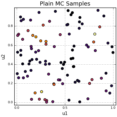 100 samples scattered across the unit square.
The variance of this (2n-sample) estimator is given by:
\[ \text{Var}[\hat{\mu}] = \text{Var}\left[\frac{1}{2n} \sum_i X_i\right] = \left(\frac{1}{2n}\right)^2 \sum_i^{2n} \text{Var}[X_i] = \frac{\sigma^2}{2n} \]
Now, the thing is that, \(\sigma^2\) is the variance of a single sample \(X_i\) and \(n\) is the total number of samples.
The variance of our estimator is \(\mathbb{E}[(\hat{\mu} - \mu)^2]\), or in other words, the “expected squared error” with respect to the true expectation \(\mu\).
We could decrease variance by increasing our sample count \(n\), but this is pretty expensive to do. While variance is proportional to \(\frac{1}{n}\), the standard deviation (which has the same units as \(\mu\) and is proportional to the confidence interval of our estimator) decreases at \(\frac{1}{\sqrt{n}}\), a far slower rate. This is not a good thing..
Instead, we’ll use variance reduction techniques to construct estimators with the same expected value as our MC estimator, but with lower variance using the same number of samples.
Antithetic Sampling
Antithetic sampling is a clever extension to the basic Monte Carlo estimator. The idea is to pair each sample \(X_i\) with an antithetic sample \(Y_i\) such that \(X_i\) and \(Y_i\) are identically distributed, but negatively correlated. So our single sample estimate is given by:
\[ \hat{\mu} = \frac{X_i + Y_i}{2} \]
Since \(\mathbb{E}[X_i] = \mathbb{E}[Y_i]\), this estimator has the same expected value as the plain MC estimator.
\[ \text{Var}[\hat{\mu}] = \frac{1}{4}\text{Var}[X_i + Y_i] = \frac{1}{4}(\text{Var}[X_i] + \text{Var}[Y_i] + 2\text{Cov}(X_i, Y_i)) = \frac{1}{2}(\sigma^2 + \sigma^2\beta) \]
Where \(\text{Var}[X_i] = \text{Var}[Y_i] = \sigma^2\) and \(\beta = \text{Corr}(X_i, Y_i) = \frac{\text{Cov}(X_i, Y_i)}{\sigma^2}\).
If we sample \(N\) of these pairs (for a total of \(2N\) samples), the variance is \(\frac{1}{2n}(\sigma^2 + \sigma^2\beta)\), and it’s easy to see that this estimator has a strictly lower variance than the plain Monte Carlo as long as \(\beta\) is negative.
Unfortunately, there isn’t a method for generating good antithetic samples. If the random sample of interest \(X_i = f(U_i)\) is a transformation of a uniform random variable \(U_i \sim \text{Uniform}(0, 1)\), we can try “flipping” the input and letting \(Y_i = f(1 - U_i)\). \(1 - U_i\) is distributed identically to \(U_i\), and assuming \(f(U_i)\) is monotonic, then \(Y_i\) will be large when \(X_i\) is small, and vice versa.
However, this assumption does not hold in general for 2D functions. In fact, for our choice of \(f(U)\), it is only slightly negatively correlated (\(\beta \approx -0.07\)).
function antithetic(N)
    u1_x = rand(N); u2_x = rand(N);
    u1_y = 1-u1_x; u2_y = 1-u2_x;
    x = f(u1_x,u2_x);
    y = f(u1_y,u2_y);
    return [u1_x; u1_y], [u2_x; u2_y], [x;y], (u1_x,u2_x,x,u1_y,u2_y,y)
end
Notice how each \(X_i\) sample (“+”) is paired with an antithetic sample \(Y_i\) (“x”) mirrored across the origin. Right?
u1,u2,x,ii=antithetic(N)
u1_x,u2_x,x,u1_y,u2_y,y = ii
scatter(u1_x,u2_x,
        m=(10,:cross),markercolor=x,
        size=(400,400),label="X samples",
        xlabel="u1",ylabel="u2",title="Antithetic Sampling")
scatter!(u1_y,u2_y,
        m=(10,:xcross),markercolor=y,
        label="antithetic samples")
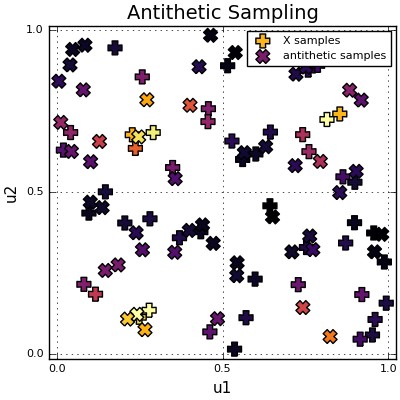 Each X sample (+) is paired with its antithetic counterpart (×) mirrored across the origin.
Control Variates
Control Variates is similar to antithetic sampling in that we’ll be pairing every sample \(X_i\) with a sample of \(Y_i\) (the “control variate”), and exploiting correlations between \(X_i\) and \(Y_i\) to decrease variance.
However, we see that \(Y_i\) is no longer sampled from the same distribution as \(X_i\). Typically \(Y_i\) is some random variable that is easy to generate from the generative process for \(X_i\). For instance, the weather report that forecasts temperature \(X\) also happens to predict rainfall \(Y\). We can use rainfall measurements \(Y_i\) to improve our estimates of “average temperature” \(\mathbb{E}[X]\).
Let’s suppose control variate \(Y\) has a known expected value \(\bar{\mu}\). So the single sample estimator is given by:
\[ \hat{\mu} = X_i - c(Y_i - \mathbb{E}[Y_i]) \]
Where \(c\) is some constant. In expectation, \(Y_i\) samples are cancelled out by \(\bar{\mu}\) so this estimator is unbiased.
Its variance is:
\[ \text{Var}[\hat{\mu}] = \text{Var}[X_i - c(Y_i - \mathbb{E}[Y_i])] = \text{Var}[X_i - cY_i] = \text{Var}[X_i] + c^2 \text{Var}[Y_i] + 2c\text{Cov}(X_i, Y_i) \]
Note: \(\mathbb{E}[Y_i]\) is not random, and has zero variance.
Calculus tells us that the value of \(c\) that minimizes \(\text{Var}[\hat{\mu}]\) is:
\[ c^* = -\frac{\text{Cov}(X_i, Y_i)}{\text{Var}(Y_i)} \]
so the best variance we can achieve is:
\[ \text{Var}[\hat{\mu}] = \text{Var}[X_i] - \frac{\text{Cov}(X_i, Y_i)^2}{\text{Var}(Y_i)} \]
The variance of our estimator is reduced as long as \(\text{Cov}(X_i, Y_i)^2 \neq 0\). Unlike antithetic sampling, control variates can be either positively or negatively correlated with \(X_i\).
The catch here is that \(c^*\) will need to be estimated. There are a couple ways:
- Forget optimality, just let \(c^* = 1\)! This naive approach still works better than basic Monte Carlo because it exploits covariance structure.
- Estimate \(c^\) from samples \(X_i\), \(Y_i\). Doing so introduces a dependence between \(c^\) and \(Y_i\), which makes the estimator biased, but in practice this bias is small compared to the standard error of the estimate.
- An unbiased alternative to (2) is to compute \(c^*\) from a small set of \(m < n\) “pilot samples”, and then throw the pilot samples away before collecting the real \(n\) samples.
In the case of our \(f(u)\), we know that the modes of the distribution are scattered in the corners of the unit square. In polar coordinates centered at \((0.5, 0.5)\), that’s about \(k\frac{\pi}{2} + \frac{\pi}{4}, k = 0, 1, 2, 3\). Let’s choose \(Y = -\cos(4\theta)\), where \(\theta\) is uniform about the unit circle.
cv(u1,u2) = -cos(4*atan((u2-.5)./(u1-.5)))
pcv = plot(linspace(0,1,100),linspace(0,1,100),cv,st=:contourf,title="Y",xlabel="u1",ylabel="u2")
plot(pcv,p0,layout=2)
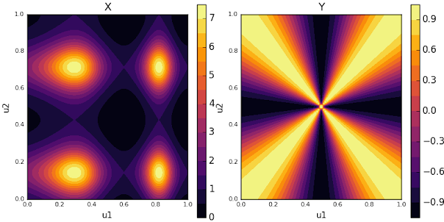 Left: our function X. Right: our control variate Y. Notice how Y’s peaks align with X’s modes.
\[ \mathbb{E}_U[Y] = \int_0^1 \int_0^1 -\cos(4\theta) \, du_1 \, du_2 = \pi - 3 \]
In practice though, we don’t have an analytic way to compute \(\mathbb{E}[Y]\), but we can estimate it in an unbiased manner from our pilot samples.
function controlvariates(N)
    # generate pilot samples
    npilot = 30
    u1 = rand(npilot); u2 = rand(npilot)
    x = f(u1,u2)
    y = cv(u1,u2)
    β=corr(x,y)
    c = -β/var(y)
    μ_y = mean(y) # estimate mean from pilot samples
    # real samples
    u1 = rand(2*N); u2 = rand(2*N)
    x = f(u1,u2)
    y = cv(u1,u2)
    return u1,u2,x+c*(y-μ_y),(μ_y, β, c)
end
We can verify from our pilot samples that the covariance is quite large:
βs=[]
for i=1:1000
    u1,u2,x,ii=controlvariates(100)
    βs = [βs; ii[2]]
end
mean(βs) # 0.367405
Stratified Sampling
The idea behind stratified sampling is very simple: instead of estimating \(\mathbb{E}[X]\) over the domain \(U\), we break up the domain into \(K\) strata, estimate the conditional expectation \(X\) over each strata separately, then average our per-strata estimates.
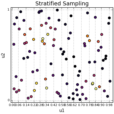 The sample space divided into 50 vertical strata, with 2 points in each.
In the above picture, the sample space is divided into 50 strata going across the horizontal axis and there are 2 points placed in each strata. There are lots of ways to stratify—you can stratify in a 1D grid, 2D grid, concentric circles with varying areas, whatever you like.
We’re not restricted to chopping up \(U\) into little fiefdoms as above (although it is a natural choice). Instead, we introduce a “stratification variable” \(Y\) with discrete values \(y_1, \ldots, y_k\). Our estimators for each strata correspond to the conditional expectations \(\mathbb{E}[X \mid Y = y_i]\) for \(i = 1 \ldots K\).
The estimator is given by a weighted combination of strata estimates with the respective probability of each strata:
function stratified(N)
    # N strata, 2 samples per strata = 2N samples
    u1 = Float64[]
    u2 = Float64[]
    for y=range(0,1/N,N)
        for i=1:2
            append!(u1, [y+1/N*rand()])
            append!(u2, [rand()])
        end
    end
    return u1,u2,f(u1,u2),[]
end
\[ \hat{\mu} = \sum_{i}^{k} p(y_i)\mathbb{E}[X \mid Y = y_i] \]
The variance of this estimator is:
\[ \sum_{i}^{k} p(y_i)^2 V_i \]
Where \(V_i\) is the variance of estimator \(i\).
For simplicity, let’s assume:
- We stratify along an grid, i.e. \(p(y_i) = \frac{1}{k}\)
- We are using a simple MC estimator within each strata, \(V_i = \frac{\sigma_i^2}{n_i}\), with \(n_i = \frac{2n}{k}\) samples each (so the total number of samples is \(2n\), the same as the plain MC estimator). \(\sigma_i^2\) is the variance of an individual sample within each strata.
Then the variance is:
\[ \sum_{i}^{k} \left(\frac{1}{k}\right) \left(\frac{k}{2n}\sigma_i^2\right) = \frac{1}{2n} \sum_{i}^{k} p(y_i)\sigma_i^2 \leq \frac{1}{2n}\sigma^2 \]
The variance within a single grid cell \(\sigma_i^2\) should be smaller than the variance of the plain MC estimator, because samples are closer together.
Here’s a proof that \(\sum_{i}^{k} p(y_i)\sigma_i^2 \leq \sigma^2\):
Let \(\mu_i = \mathbb{E}[X \mid Y = y_i]\) and \(\sigma_i^2 = \text{Var}[X \mid Y]\)
Using the tower property:
\[ \mathbb{E}[X^2] = \mathbb{E}Y[\mathbb{E}_X[X^2 \mid Y]] = \sum{i}^{k} p(y_i)\mathbb{E}[X^2 \mid Y = y_i] = \sum_{i}^{k} p(y_i)(\sigma_i^2 + \mu_i^2) \]
via \(\text{Var}[X \mid Y] = \mathbb{E}[X^2 \mid Y] - \mathbb{E}[X \mid Y = y_i]^2\)
\[ \mathbb{E}[X] = \mathbb{E}Y[\mathbb{E}_X[X \mid Y]] = \sum{i}^{k} p(y_i)\mu_i \]
\[ \sigma^2 = \mathbb{E}[X^2] - \mathbb{E}[X]^2 = \sum_{i}^{k} p(y_i)\sigma_i^2 + \left[\sum_{i}^{k} p(y_i)\mu_i^2 - \left(\sum_{i}^{k} p(y_i)\mu_i\right)^2\right] \]
Note that the term \(\sum_{i}^{k} p(y_i)\mu_i^2 - \left(\sum_{i}^{k} p(y_i)\mu_i\right)^2\) corresponds to the variance of a distribution that takes value \(\mu_i\) with probability \(p(y_i)\). This term is strictly non negative, and therefore the inequality \(\sum_{i}^{k} \frac{k}{2n}\sigma_i^2 \leq \sigma^2\) holds.
This yields an interesting observation: when we do stratified sampling, we are eliminating the variance between strata means. This means that we get the most gains by choosing strata such that samples vary greatly between strata.
Here’s a comparison of the empirical vs. theoretical variance with respect to number of strata:
# theoretical variance
strat_var = zeros(50)
for N=1:50
    sigma_i_2 = zeros(N)
    y = range(0,1/N,N)
    for i=1:N
        x1 = y[i].+1/N*rand(100)
        x2 = rand(100)
        sigma_i_2[i]=var(f(x1,x2))
    end
    n_i = 2
    strat_var[N] = sum((1/(N))^2*(1/n_i*sigma_i_2))
end
s = estimatorVar(stratified)
plot(1:50,s,label="Empirical Variance",title="Stratified Sampling")
plot!(1:50,strat_var,label="Theoretical Variance")
Some random thoughts about this
-
Stratified Sampling can actually be combined with other variance reduction techniques. What I mean by this, when computing the conditional estimate within a strata, we free to use antithetic sampling, control variates within the strata. You can even do stratified sampling within your strata. This makes sense if your sampling domain is already partitioned into a bounding volume hierarchy, such as a KD Tree.
-
Antithetic sampling can be regarded as a special case of stratified sampling with 2 strata. The inter strata variance you are eliminating here is the self symmetry in the distribution of \(X\) (the covariance between one half and another half of the samples). Anyway, I’ll stop from here. Do note I am skipping the standard deviations of these estimators but I will soon post it here when I have time. I really hope you enjoy reading this post, as much as I had making it. It really helps me explaining it to the outside world as it tests what I know and what I don’t know.